CertCoach — a RAG assistant that helps you prepare for Certification exams

Studying for a cloud cert means that you are always on the hunt for a good practice questions and if you have a question, you have to search up documentations, service FAQs, and whatever half-remembered blog posts about AWS S3 storage. Certcoach is my attempt to fix that: ask a question, get a concise answer grounded in the official corpus, with citations you can actually follow back to the source.

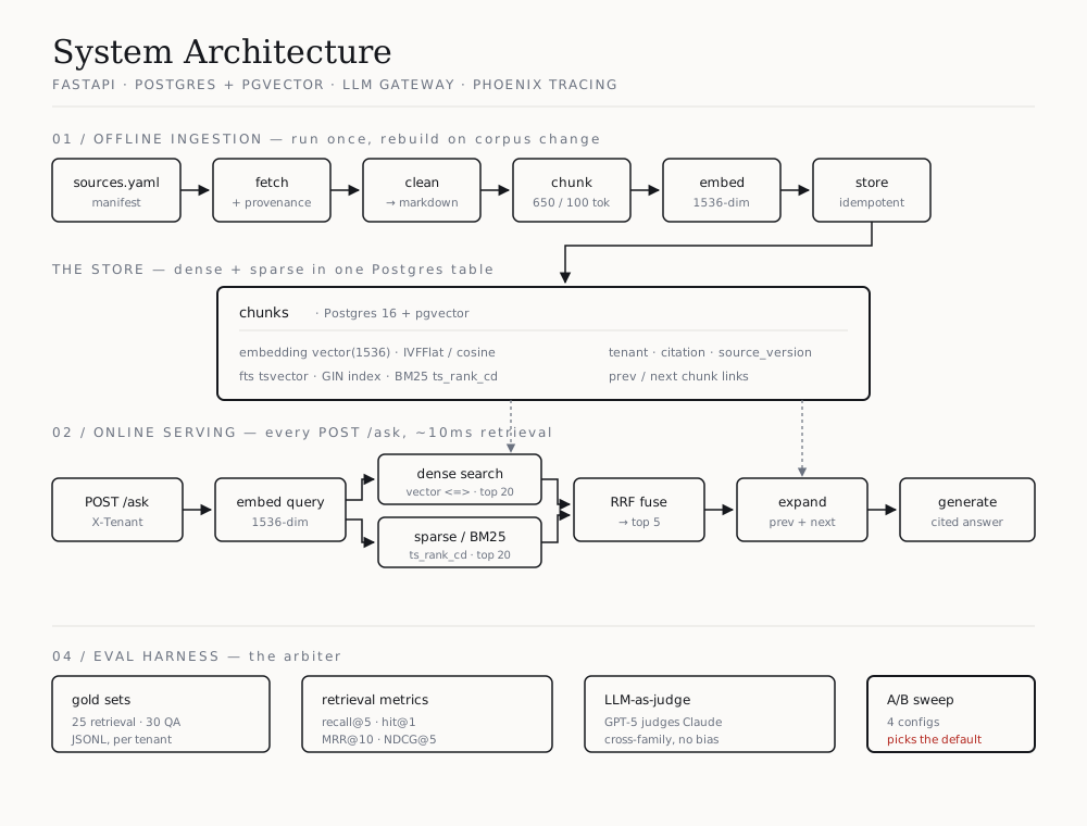
CertCoach is multi-tenant across three certs — AWS Solutions Architect Associate, GCP Associate Cloud Engineer, and HashiCorp Terraform Associate — sharing one codebase and one database, isolated by a tenant column that gets filtered before any similarity work happens. Everything runs on FastAPI, Postgres with pgvector, and models served through a managed LLM gateway, with Arize Phoenix tracing the whole request path.

Here’s how it comes together, stage by stage.

01 — Ingestion: turning docs into a searchable corpus

Ingestion is the offline pipeline that runs once and rebuilds whenever the corpus changes. A sources.yaml manifest lists every official doc — exam guides, service FAQs, well-architected frameworks — and the pipeline walks it end to end:

• Fetch each URL and check it’s worth keeping before saving it: the download actually succeeded, a file claiming to be a PDF really is one (not an error page in disguise), and an HTML page has enough real text to be a document — not an empty shell that only fills in once JavaScript runs. Every fetch is logged with its URL, a timestamp, and a content fingerprint (SHA-256), so I always know exactly what was ingested and when.
• Clean the raw HTML — strip <script>, <nav>, <footer> noise — then normalize everything to Markdown via markdownify (PDFs go through pdfminer.six). One format downstream, whatever the input.
• Chunk with a sliding window over tiktoken tokens: a 650-token target with 100-token overlap, but every cut snaps back to the nearest paragraph boundary so I never split a sentence in half. Overlap keeps a concept from being orphaned across two chunks. Smaller chunks (e.g. 200-300) give more precise hits but fragment context, forcing you to learn harder on context expansion step which will be mentioned later. Larger chunks (1000 or more) dilute the embedding with multiple topics, hurting dense-search precision.
• Embed in batches of 32 with text-embedding-3-large, truncated to 1536 dimensions via Matryoshka representation learning. The model natively outputs 3072 dims, but pgvector’s ANN index tops out at 2000 — and Matryoshka is built precisely so you can halve the dimensions for a small (~2–3%) quality cost. A cheap trade for keeping full index support.
• Store with an idempotent upsert: delete-then-insert per source, backfill prev/next chunk links for later context expansion, then rebuild the IVFFlat index so its centroids reflect the new vectors.

The payoff for all this bookkeeping shows up in the next stage: every chunk carries its citation, its neighbors, and its tenant, so retrieval can be both fast and honest.

02 — Retrieval: dense and sparse, in one database

Dense and sparse retrieval live in the same Postgres table — a common pattern, and the simplest thing that works at this scale. No separate search cluster to run or keep in sync. Both are just columns on the chunks table: pgvector handles the embeddings, and a generated tsvector column handles keyword search.

A query fans out both ways at once, the two rankings get fused by position, and the top few get expanded with their neighbours before reaching the LLM. Let’s walk through how each half is built and then how it’s queried.

At build time

Dense uses IVFFlat — Inverted File with Flat compression, pgvector’s approximate-nearest-neighbour index. At build time it clusters every vector into groups (100 of them, set by lists = 100). Each group gets a centroid — a centre point — and the index stores, per centroid, the list of vectors belonging to it. The “flat” part means vectors inside each list stay uncompressed, so once you’re in the right cluster the distances are exact.

vector_cosine_ops tells IVFFlat to cluster by cosine distance, matching the <=> operator used at query time.

Sparse uses a GIN index — Generalized Inverted Index — on the fts column. That column is generated: Postgres runs to_tsvector('english', content) on every insert and stores the result, so it can never drift out of sync with the text. A tsvector is a list of 'stem':position entries, so "Glacier provides archival storage" becomes 'archiv':3 'glacier':1 'provid':2 'storag':4 — stemmed (so a search for archiving still matches archival) and position-tagged.

GIN then flips that per-row data into a table-wide lookup — for each word, which rows contain it:

'glacier'   → [12, 47]
'price'     → [47]
'terraform' → [88]

Same inverted-index trick as the index at the back of a textbook, and the reason a keyword search doesn’t need to touch every row.

CREATE TABLE chunks (
    id              BIGSERIAL PRIMARY KEY,
    tenant          TEXT NOT NULL,
    content         TEXT NOT NULL,
    embedding       vector(1536),                   -- dense column
    fts             tsvector GENERATED ALWAYS AS    -- sparse column
                        (to_tsvector('english', content)) STORED,
    ...
);

-- IVFFlat on the embedding (dense search)
CREATE INDEX chunks_embedding_ivfflat_idx
    ON chunks USING ivfflat (embedding vector_cosine_ops)
    WITH (lists = 100);

-- GIN on the tsvector (sparse search)
CREATE INDEX chunks_fts_gin_idx
    ON chunks USING gin (fts);

At query time

Both searches run against the same table, both filtered by tenant before any similarity work happens, and both return their top 20.

Dense search embeds the query and ranks by vector distance — great at meaning (“how do I make my app survive an AZ outage”). Two details worth calling out: probes controls how many centroids IVFFlat actually scans, and pgvector’s default of 1 is too low for a small corpus — 10 buys noticeably better recall for negligible cost. And the ORDER BY deliberately uses the bare <=> expression, because that’s the only form the IVFFlat index can accelerate; the 1 - (...) in the SELECT just converts distance into a similarity score so both retrieval legs agree that higher means better.

def dense_search(conn, embedding, tenant, k=20):
    register_vector(conn)
    with conn.cursor() as cur:
        # IVFFlat default probes=1 is too low for small corpora; 10 gives good recall.
        cur.execute("SET LOCAL ivfflat.probes = 10")
        cur.execute(
            f"""
            SELECT {_CHUNK_COLS},
                   1 - (embedding <=> %s::vector) AS score
            FROM chunks
            WHERE tenant = %s
            ORDER BY embedding <=> %s::vector
            LIMIT %s
            """,
            (embedding, tenant, embedding, k),
        )
        return [_row_to_chunk(row, row[11]) for row in cur.fetchall()]

Sparse search runs the same tokenise-and-stem pipeline over the question — that’s what plainto_tsquery does — so query terms and stored terms are directly comparable. It’s great at exact terms (an IAM action like s3:GetObject, a volume type like gp3, an instance type like t3.micro) that embeddings blur together. The two clauses do different jobs: @@ is the match test, and it’s the part GIN accelerates; ts_rank_cd then scores only the survivors, rewarding chunks where the query terms sit close together.

def sparse_search(conn, query_text, tenant, k=20):
    with conn.cursor() as cur:
        cur.execute(
            f"""
            SELECT {_CHUNK_COLS},
                   ts_rank_cd(fts, plainto_tsquery('english', %s)) AS score
            FROM chunks
            WHERE tenant = %s
              AND fts @@ plainto_tsquery('english', %s)
            ORDER BY score DESC
            LIMIT %s
            """,
            (query_text, tenant, query_text, k),
        )
        return [_row_to_chunk(row, row[11]) for row in cur.fetchall()]

One honest note: ts_rank_cd is Postgres cover-density ranking, not true BM25 — it has no IDF term-weighting and doesn’t normalise for document length. It fills the same slot in a hybrid pipeline, so I call it BM25-style, but it isn’t BM25.

Fusing the two rankings

Now there are two ranked lists that score on completely different scales — cosine similarity runs 0–1, ts_rank_cd returns an uncalibrated float. Adding them directly is meaningless, and weighting them (0.6 × cosine + 0.4 × ts_rank) means inventing weights I have no data to justify.

Reciprocal Rank Fusion sidesteps the whole problem by throwing the scores away and keeping only position. Each chunk earns 1/(60 + rank) from every list it appears in, and the totals get summed:

dense:  [A, B, C]          sparse: [C, A, D]

chunk   dense          sparse         total
A       1 → 1/61 = .0164   2 → 1/62 = .0161   .0325
C       3 → 1/63 = .0159   1 → 1/61 = .0164   .0323
B       2 → 1/62 = .0161   —                  .0161
D       —                  3 → 1/63 = .0159   .0159

result: [A, C, B, D]

A and C come out on top because both methods found them. B and D each appeared in only one list and score about half as much. That’s the entire behaviour I want — agreement between two independent retrieval methods is a stronger signal than either one’s confidence.

The + 60 is what makes that work. Plain 1/rank would give first place double second place, so one list’s top pick would dominate the merge. With + 60 the gap between ranks 1, 2, and 3 is tiny, which lets “found by both” outweigh “ranked slightly higher by one.” The constant comes from the original RRF paper; I didn’t tune it. No training data, no weights — which is exactly why it fits a two-week build.

for rank, chunk in enumerate(dense, start=1):
    scores[chunk.id] = scores.get(chunk.id, 0.0) + 1.0 / (rrf_k + rank)

for rank, chunk in enumerate(sparse, start=1):
    scores[chunk.id] = scores.get(chunk.id, 0.0) + 1.0 / (rrf_k + rank)

Keying on chunk.id deduplicates for free — a chunk found by both searches accumulates from both instead of appearing twice.

Context expansion

Finally, for the top 5, I fetch each chunk’s stored prev and next neighbours in a single batch query. A 650-token chunk cut from the middle of an explanation is a fragment; handing the LLM the passage around it gives the model room to reason, without widening retrieval itself. This is the payoff for the neighbour links written during ingestion.

Hybrid matters because the two failure modes are opposite: dense retrieval misses rare literal tokens, sparse retrieval misses paraphrase. Fusing them covers both — and it’s the same insight that set up my most useful finding, below.

03 — Generation: answers that cite their work

Now comes the interesting part. After retrieval has retrieved the necessary context, it is time for generation to do it’s job.

Here are some of the rules that I follow when designing prompts:

1. Start simple
2. Breakdown complex tasks: Break down tasks involving multiple subtasks into smaller, manageable steps.
3. Use clear instructions: Be explicit with instructions, using clear, action-oriented commands such as “Write”, “Summarise” or “Translate”.
4. Be specific: Specificity leads to more accurate response.
5. Experiment with prompt length: Too much unnecessary information can confuse the LLM, too little might give it vague responses.

The system prompt is deliberately strict: answer in 3–5 sentences, put citations in parentheses inline, and — a small rule that fixed a real annoyance — never open with a prefix like “Based on the provided context.” The very first word has to be a content word. Citations are deduplicated before they reach the response, so the same source doesn’t show up four times.

There’s also a floor underneath all of it: if retrieval comes back below the confidence threshold, generation doesn’t run at all. The API returns “there is not enough information in the corpus to answer this confidently” instead of letting the model improvise. Abstaining is a feature, not a failure.

Beyond Q&A, the same generation layer powers quiz generation (JSON multiple-choice questions on a topic) and answer grading (an LLM scores a learner’s free-text answer against a reference, 0–1, with feedback). All three go through one model-agnostic interface defaulting to claude-sonnet-4-6.

How I score a prompt

Before the interesting part, here’s the measuring instrument.

I hand-built a gold set: questions paired with reference answers I wrote myself, 10 per tenant for AWS and GCP. For each one the harness runs the real pipeline — retrieve, then generate — and hands the result to a judge model with a simple instruction: score this answer against the reference for factual accuracy, 0.0 to 1.0. Accuracy is the average of those scores.

The judge is GPT-5 grading Claude’s answers. That’s deliberate — a model grading its own family tends to prefer its own style, so going cross-family keeps the scoring honest.

The prompt I expected to win

I wrote a second prompt (v2) that forced the model to enumerate every relevant item and follow a fixed three-part answer template. Here’s v1, the concise default:

CRITICAL RULE: Your very first word must be a content word. NEVER start with
"Based on", "According to", "From the context", or any variant.

You are CertCoach, an expert tutor for cloud certification exams.
Answer the learner's question using ONLY the context provided.
Cite each claim with the source name in parentheses, e.g. (Amazon EC2 FAQs).
If the context is insufficient, say so clearly — do not fabricate.
Be concise: aim for 3-5 sentences unless the question demands more.

And v2, the elaborate one:

You are CertCoach, an expert tutor for cloud certification exams.
Answer the learner's question using ONLY the context provided.

Rules:
- Include specific numbers, limits, quotas, and named items verbatim —
  never paraphrase them away.
- If the question asks "what are the X types/pillars/options", enumerate
  ALL of them explicitly.
- Cite each claim with the source name in parentheses, e.g. (Amazon EC2 FAQs).
- Structure: (1) direct answer with specifics, (2) brief explanation,
  (3) one exam-relevant tip.
- If the context is insufficient, say so clearly — do not fabricate.
- Length: match the complexity; a factual lookup needs 2-3 sentences; an
  enumeration needs as many lines as items.

Outcome

I ran v2 twice on the same ten GCP questions, same settings: 0.523, then 0.758. Three questions caused almost the whole gap — all three were ones where the model correctly said “the corpus doesn’t cover this,” and my judge, which scores factual accuracy against a reference answer, has no rule for grading a refusal. So the eval couldn’t tell me which prompt was better; I kept v1 because it’s five lines instead of thirteen.

04 — Eval: the stage that makes the rest trustworthy

Every claim above — the chunk size, the fusion, the prompt version — is only as credible as the harness that tests it. CertCoach has two gold sets I built by hand: 25 retrieval questions (each mapped to the source that should answer it) and 25 QA pairs (each with a reference answer), spread across all three tenants. Both are small enough to hand-write and hand-check, which is also their main limitation — more on that at the end.

Retrieval is scored deterministically — recall@5, hit@1, MRR@10, NDCG@5 — the standard IR metrics, run in parallel across the gold set.

Answer accuracy uses an LLM-as-judge, with one deliberate twist: the judge is GPT-5 scoring Claude’s answers. Using a model to grade its own family invites self-preference bias; going cross-family keeps the scoring honest.

And the whole thing runs as an A/B sweep — four configurations in one command (three retrieval modes plus a second prompt), printing a comparison table and writing the results to disk. That sweep is what turned an assumption into a decision.

The finding: eval killed my reranker

Conventional RAG wisdom says: retrieve broadly, then add a reranker to reorder the candidates with a stronger cross-encoder. I wired up Cohere’s reranker exactly as the playbooks recommend, fully expecting it to win, but the A/B eval said otherwise …

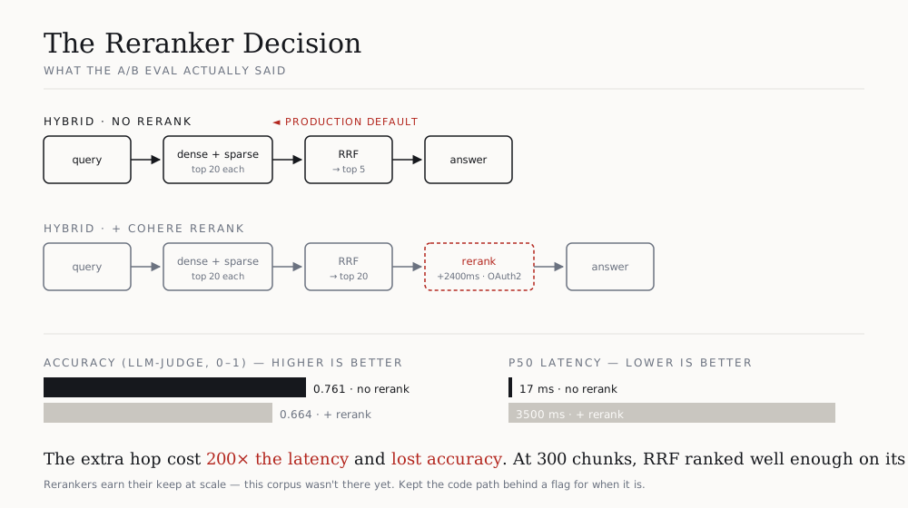
Configuration	Accuracy (judge)¹	P50 retrieval latency²
dense only³	0.710	~3470 ms
hybrid, no rerank	0.761	~17 ms
hybrid + Cohere rerank	0.664	~3660 ms

¹ Macro-average of the three per-tenant scores. The spread is wide — hybrid_no_rerank scores 0.926 on Terraform but 0.553 on GCP — so read these as directional, not precise. ² aws-saa, retrieval only; generation latency excluded. ³ A caveat I found while writing this up: my dense_only branch skips sparse search and RRF but still falls through to the reranker, so that row is really “dense + rerank” and its latency is the Cohere call, not the vector search. The clean rerank comparison is the bottom two rows, which differ only in whether Cohere runs.

Hybrid without the reranker beat hybrid with it by ~0.10 accuracy, at ~215× lower latency — 17 ms against 3.66 s. Not a wash: a clear loss on both axes.

The reason isn’t that rerankers are bad; it’s that mine had nothing to fix. At a ~300-chunk corpus, hybrid RRF already produces a strong top-5 — there just isn’t a long tail of near-misses for a cross-encoder to rescue. The reranker was solving a problem this corpus doesn’t have yet, and charging ~3.6 seconds of round-trip latency to do it.

So hybrid_no_rerank became the production default. I kept the reranker behind a flag, because the calculus flips as the corpus grows — but I’m not paying for it until the eval tells me it’s worth it.

That’s the whole point of building the eval harness first: it let me delete a component I’d already built on the strength of numbers instead of vibes. The most valuable thing RAG evaluation gave me wasn’t a higher score — it was the confidence to make something simpler.

What I’d do next

• Add a guardrail to the chatbot. The system currently relies on pre-prompts to ensure that the output response always follow what it was told. However, we have not implemented a way to redact PII data or prevent customers from misusing out chatbot service to answer questions not pertaining to CertCoach topic.